Key takeaways
- Low voltage is the inverter output, 600 to 690 V in one datasheet.
- Our 20 MWac feeder carries 334.7 A at 34.5 kV and 577.4 A at 20 kV. One 4.0 MVA station on the LV side carries 3,347 A at 690 V.
- For the same conductor and power, loss scales with 1 over voltage squared. A 500 kcmil feeder loses 81.6 kW at 34.5 kV and 242.8 kW at 20 kV, a ratio of 2.98.
- With cable sized to ampacity, full-load loss is 113.3 kW (0.57%) at 34.5 kV and 149.0 kW (0.74%) at 20 kV.
- Generation raises voltage along the feeder. At unity power factor the far station sits 0.85% above the substation at 34.5 kV and 1.24% above at 20 kV.
To lay out and size an MV and LV network in software, see the best utility-scale solar design software.
MV/LV design at a glance
MV/LV design fixes the voltage of each AC circuit between the inverter and the grid connection. It then sizes cable, switchgear and transformers to match. The table gives the formulas and ranges.
| Item | Detail |
|---|---|
| Formula | Current I = S ÷ (√3 × V). Loss = 3 × I² × R × L. Voltage change ≈ √3 × I × (R cos φ ± X sin φ) × L ÷ V. |
| Unit / typical range | LV 600 to 690 V and MV 12 to 36 kV in the FIMER PVS980-MVP datasheet. SMA lists 13 MV options from 10.0 to 34.5 kV. No source read gives a single definition of MV. |
| Where it matters | Collector layout, cable schedule, single-line diagram, loss budget and the grid connection. |
| Standard or rule | Not the standard text. Limits come from the project, the utility and the equipment maker. |
| In software | Layout tools draw MV and LV networks. Electrical tools size cable and report loss or drop (see the table below). |
Why does MV/LV design matter for installers and EPCs?
The voltage you pick sets the current. Current sets cable size, loss and voltage rise. None is easy to change once the layout is fixed.
Cable cross-section is metal you buy. Loss is energy you do not sell. A feeder near its ampacity has no margin. In our example the 20 kV head cable runs at 99.5% of its datasheet rating.
An NREL paper on a wind plant (January 2006) says collector design seeks to minimise losses and voltage drops within budget limits. It says full-load losses may range from 1.5% to 3%. That is a wind plant, so read it as context, not a PV target. Our short feeder gives less.
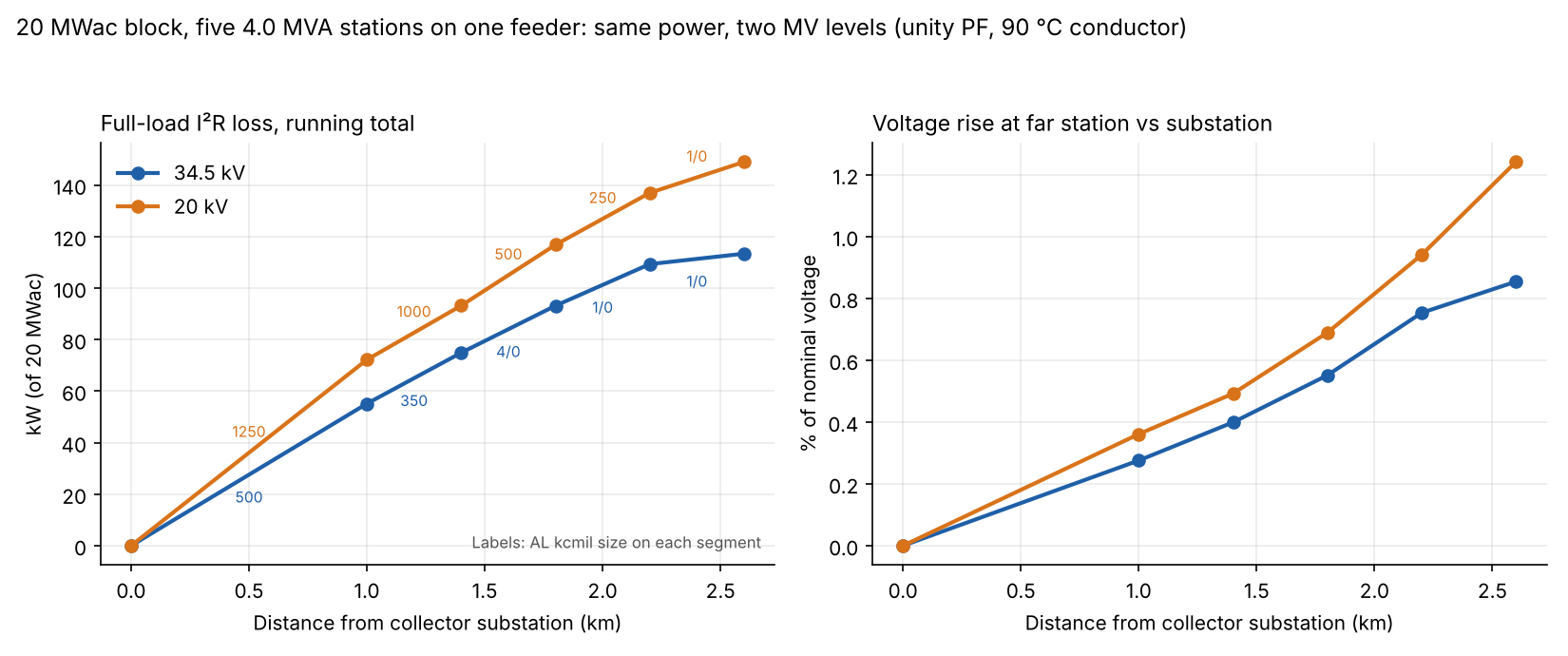
Figure 1. At the same 20 MWac, the 20 kV feeder loses 149.0 kW against 113.3 kW. Its far station also rises more: 1.24% against 0.85%.
Where does LV end and MV begin in a solar plant?
In a station-type layout, LV ends at the low-voltage terminals of the inverter transformer. Everything from its MV side to the collector substation is MV. Plants with string inverters or other layouts may place the boundary elsewhere.
- LV side: inverter AC output and the cable to the transformer. FIMER’s datasheet lists 600, 630, 660 and 690 V. At 4.0 MVA that is 3,347 A at 690 V, which is 50 times the 66.9 A at 34.5 kV. At 600 V it is 3,849 A. The loss in the same conductor at the same power would be 2,500 times higher at 690 V than at 34.5 kV, because loss follows current squared.
- Transformer: FIMER lists an oil-immersed, outdoor unit rated equal to the station, from 1,818 to 4,182 kVA. See transformer.
- MV switchgear and feeders: FIMER’s SF6 ring main unit is rated 540 A at 50 °C (nominal 630 A). A feeder that daisy-chains through such switchgear would go over that rating at 20 kV (577.4 A). It would not at 34.5 kV (334.7 A). Layout decides whether it does.
- Collector substation: feeders meet the main transformer. One AES design-criteria document (Revision C, 14 June 2021) gives 34.5 kV nominal and 36.3 kV maximum for its collector system. See substation design and the single-line diagram.
Why choose one MV level over another?
A higher voltage cuts current in proportion. It cuts loss in a fixed conductor by the voltage ratio squared. The level is rarely free, because equipment and the utility limit the options.
SMA’s MV station document lists 13 nominal options from 10.0 to 34.5 kV, including 20.0 and 34.5 kV. FIMER’s datasheet gives 12 to 36 kV. Agree the interconnection voltage with the utility early. See interconnection application.
No source read compares voltage levels or says why 34.5 kV is common. The comparison below is arithmetic on a stated block. Cable and switchgear are not priced. So a lower loss at 34.5 kV is not a total cost result.
How do you calculate feeder current, loss and voltage change?
Find the current in each feeder segment and pick a cable that carries it. Then sum loss and voltage change. These steps cover a radial feeder.
- Station current: I = S ÷ (√3 × V), where S is in volt-amperes and V is line to line.
- Segment current: the number of stations beyond the segment times I. The head segment carries the whole block.
- Cable: take the smallest size whose datasheet ampacity covers the segment current. This is a screen, not a thermal study. The model leaves out soil, depth and grouping. See wire and conductor sizing.
- Loss: 3 × I² × R × L per segment, where R is the AC resistance at 90 °C in ohm per km.
- Voltage change: √3 × I × (R cos φ + X sin φ) × L ÷ V, summed along the feeder. Take sin φ as positive when the plant exports reactive power. That raises the voltage. Absorbing reactive power lowers it. A complex-impedance solver agreed within 0.03 percentage points.
- Transformer loading: station apparent power divided by the transformer rating.
For the resistance-only method on DC and LV runs, see voltage drop calculation. For reactive power and kVA limits, see power factor and reactive power.
Worked example: a 20 MWac block at 34.5 kV and 20 kV
Five 4.0 MVA stations on one radial feeder give 20 MWac. We use the same cable family at both voltages so that only voltage changes. Every figure is computed from the stated inputs.
| Input | Value |
|---|---|
| Block | Five stations of 4.0 MVA, unity power factor, 20 MWac in total. Assumed. |
| Layout | First station 1.0 km from the collector substation, then 0.4 km between stations, 2.6 km in total. Assumed. |
| System | Three-phase, 60 Hz, line voltage held at nominal, 34.5 kV and 20 kV. |
| Cable | Southwire SPEC 46715, AL Compact 35kV TRXLPE 133% IL, Type MV-105 single-conductor aluminium, revision 1.000.006, updated 4 June 2025. US product, 60 Hz. |
| Cable values | Table 2 as printed, 1/0 to 1250 kcmil: resistance and duct ampacity at 90 °C, reactance at 60 Hz. |
| Simplification | A 35 kV-class cable is used at 20 kV so that only voltage changes. |
A real 20 kV job would use a 20 kV-class cable with different reactance. Resistances were converted from ohm per 1,000 ft by dividing by 0.3048. The duct ampacity column is a screen only. The product title says For Direct Burial, but the datasheet gives no direct-burial ampacity.
The results below compare the same 20 MWac block at the two voltages.
| Result (full load, 90 °C) | 34.5 kV | 20 kV |
|---|---|---|
| Current per station | 66.9 A | 115.5 A |
| Feeder head current | 334.7 A | 577.4 A |
| Cable per segment, substation end first | 500, 350, 4/0, 1/0, 1/0 kcmil | 1250, 1000, 500, 250, 1/0 kcmil |
| Head cable ampacity used | 94.3% | 99.5% |
| I²R loss | 113.3 kW (0.57%) | 149.0 kW (0.74%) |
| Voltage rise at far station, unity power factor | 0.85% | 1.24% |
| Conductor index (aluminium: cross-section × length, three phases, summed over segments) | 1,230 mm²·km | 3,028 mm²·km |
The 20 kV column is indicative only, because it uses a 35 kV-class cable. With one 500 kcmil cable on every segment, loss is 81.6 kW at 34.5 kV and 242.8 kW at 20 kV. The ratio is 2.98, equal to (34.5 ÷ 20) squared (2.98). At 20 kV that cable would run at 163% of its ampacity, so it fails.
Once each level gets a cable that passes ampacity, the loss gap shrinks to 1.31 times. The cost moves into metal, as the 20 kV feeder has 2.46 times the cross-section. The conductor index is the cross-section times the length of every segment, for three phases. It is a metal measure, not a price.
Reactive power changes the voltage. At 0.95 power factor the far-station rise is 0.96% (34.5 kV) and 1.55% (20 kV) when the plant exports vars. It is 0.67% and 0.81% when it absorbs them.
Full-load loss uses the 90 °C resistance, so it overstates the loss of a cooler cable. The annual loss share depends on the output profile. See 8760 hourly simulation.
Transformer loading. Each station has a 4.0 MVA transformer. Loading is apparent power over rating, so reactive power counts.
| Case | MW | Mvar | MVA | Loading of 4.0 MVA unit |
|---|---|---|---|---|
| Unity power factor, full output | 4.00 | 0.00 | 4.00 | 100.0% |
| 0.95 power factor, 4.0 MW | 4.00 | 1.31 | 4.21 | 105.3% |
| 0.95 power factor, held at rating | 3.80 | 1.25 | 4.00 | 100.0% |
At 0.95 the station must give up 0.2 MW, capping output at 3.8 MW, or use a larger transformer. Transformer losses are not modelled, because the datasheets read do not state them. Cable length follows the layout. See utility-scale layout optimisation.
MV feeder calculator
Enter stations, rating, power factor, two voltages, distances and the transformer rating. It gives the tables above and warns when no listed cable fits.
How solar software handles MV/LV design
On the company pages read in October 2026, no tool states all three things MV design needs. Those are an editable MV and LV network, cable sizing from current and a loss or voltage figure per run. Each tool covers part of the job.
| Software | MV/LV network in the design | Cable loss or voltage drop |
|---|---|---|
| RatedPower | Yes | Not stated |
| PVcase Ground Mount | Not stated | Yes, for LV cables |
| PVsyst | Partly: MV and HV transformer losses. No MV network input described | Partly: AC wiring loss from wire length, section and metal |
| ETAP | Partly: models "collector systems" | Yes (voltage drop) |
Not stated: the company pages read do not say. It applies to RatedPower cable loss and PVcase MV networks. Partly: the page covers only part of the item.
- RatedPower: homepage (undated) says you can "refine MV and LV connections". It does not mention cable sizing or losses. Its methodology PDF is not covered here.
- PVcase Ground Mount: help page "Cable sizing", updated 28 July 2026. Covers DC string, DC main and AC cabling as low voltage. Each segment has a user-set drop limit. MV is not mentioned.
- PVsyst: help page "Ohmic losses" (undated). Transformer loss uses nominal copper loss from datasheets. Reactive losses are not modelled.
- ETAP: cable sizing page (undated): voltage drop is a sizing criterion. PV array page: models "solar combiners and collector systems". Neither page mentions medium voltage.
For a ranked comparison of tools for plant-scale design, see the best utility-scale solar design software.
Common mistakes with MV/LV design
FAQs
What voltage counts as medium voltage in a solar plant?
No source read gives one definition. FIMER’s datasheet lists 12 to 36 kV. SMA offers 10.0 to 34.5 kV. The AES criteria document uses 34.5 kV nominal. Confirm the level with the utility.
Why do many plants collect at 34.5 kV?
A higher voltage means less current, so cable is smaller and loss is lower. One 500 kcmil cable carries the 334.7 A head current of a 20 MWac block at 34.5 kV. At 20 kV the head needs 1250 kcmil, run at 99.5% of its rating. The sources read do not say why that level is common.
Does voltage rise or drop on a solar feeder?
It rises toward the generators when the plant exports power. In our example the far station is 0.85% above the substation at 34.5 kV and unity power factor. Absorbing reactive power at 0.95 lowers it to 0.67%.
How do you calculate current on an MV feeder?
Use I = S ÷ (√3 × V). A 4.0 MVA station carries 66.9 A at 34.5 kV and 115.5 A at 20 kV. Our calculator does this for every station. It does not replace a cable study. It picks cable from datasheet ampacity only. It leaves out soil heat, short-circuit rating, protection, harmonics and the transformer’s own impedance and loss.
Related terms
- Single-line diagram: the drawing that shows each MV and LV voltage level.
- Transformer: the step-up unit that marks the LV to MV boundary.
- Substation design: where the feeders meet the main transformer.
Next step: run your own block through the calculator above, then compare tools that can draw the same feeder in the best utility-scale solar design software list.
Sources
- Southwire SPEC 46715, AL Compact 35kV TRXLPE 133% IL, revision 1.000.006, updated 4 June 2025 (checked October 2026).
- FIMER PVS980-MVP datasheet, Rev B, 31 March 2021 (checked October 2026).
- SMA MVS-STP-10-TA-en-11, version 1.1 (checked October 2026).
- Riverside Solar 115 kV and 34.5 kV design criteria, Revision C, 14 June 2021 (checked October 2026).
- NREL/CP-500-38940, Equivalencing the Collector System of a Large Wind Power Plant, January 2006 (checked October 2026).
- PVcase help, Cable sizing, updated 28 July 2026 (checked October 2026).
- PVsyst help, Ohmic losses, undated (checked October 2026).
- RatedPower homepage, undated (checked October 2026).
- ETAP cable sizing and ETAP photovoltaic array, both undated (checked October 2026).
Last updated 30 October 2026. Next scheduled review: 30 January 2027.