Key takeaways
- Our example gave 10,938 kWh AC a year, or 1,367 kWh per kWdc. It used pvlib 0.16.1, with an 8 kWdc south-facing array at 25 degrees tilt.
- The weather was the Greensboro, NC TMY3 file bundled with pvlib. A hand formula on the same weather gave 10,838 kWh, 0.9% lower.
- The small gap hides offsets. Transposition added 353 kWh. Angle-of-incidence loss, cell temperature and the inverter curve took off 253 kWh.
- TMY3 stamps mark the end of each hour. If you use the stamp as the instant, annual AC changes by -0.6% south, -4.5% east and +4.1% west.
- pvlib is code, not a design tool. It has no GUI, layout or proposal module.
For tools that run a yield model without code, see the best solar simulation software. For open-source design tools, see the best open-source solar design software.
pvlib python at a glance
pvlib is a toolbox for people who write code. The docs FAQ calls it "more of a toolbox or a framework to use to build your own modeling process".
| Item | Detail |
|---|---|
| What it is | Python library of PV performance functions and classes, used through code "instead of via a GUI" (docs FAQ). |
| Version we ran | 0.16.1, which the What’s New page dates 26 September 2026. It needs Python 3.11 or newer (package metadata). |
| Example result | In the worked example, version 0.16.1 returned 10,938 kWh AC for one year from an 8 kWdc array. |
| Licence | BSD-3-Clause, as printed in the installed package’s licence file. |
| Typical inputs | Site latitude and longitude, array tilt and azimuth, module and inverter parameters, hourly or finer weather. |
| Typical outputs | Solar position, plane-of-array irradiance, cell temperature, DC and AC power as time series. |
Why does pvlib matter for installers?
pvlib lets an engineer build and inspect a yield model that no company controls. That suits internal tools, batch studies and checks of other tools’ output. It does not suit a team with no one who codes.
Wikipedia names some company users, but it is a secondary source. Installer-side uses are our view, not survey data: a quote-checking script, a batch run over many sites, or a cross-check of a design tool’s yearly figure.
The docs FAQ adds two warnings: it is "on you as the user to understand the models you are using". and pvlib "does not prevent you from using models improperly and generating invalid results".
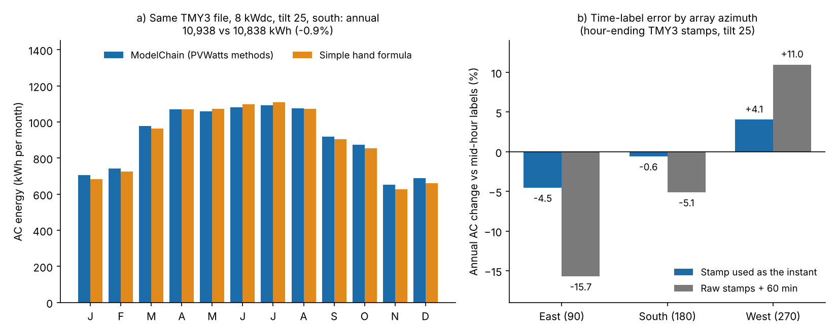
Figure 1. A hand formula landed within 0.9% of the ModelChain year, yet an hour-ending stamp used as the instant moved an east-facing array by 4.5%.
What does pvlib provide?
pvlib gives you the model steps between weather data and AC power. They come as separate functions and as one chained workflow called ModelChain. We checked the module list of the installed 0.16.1 package. A module being there says nothing about its accuracy.
- Solar position and clear sky: modules solarposition, atmosphere and clearsky.
- Irradiance: irradiance (transposition to the tilted plane and splitting global into direct and diffuse), iam (angle-of-incidence loss) and albedo.
- Temperature, module and inverter: temperature, pvsystem, singlediode, ivtools and inverter.
- Other effects: shading, soiling, snow, bifacial and tracking.
- Weather data: iotools has readers such as read_tmy3 and read_epw. It also has downloaders such as get_pvgis_tmy and get_nsrdb_psm4_tmy. See NSRDB and Meteonorm.
ModelChain runs these steps in order. The ModelChain guide lists them. They are solar position and inputs, angle-of-incidence loss, spectral loss, effective irradiance, then cell temperature, DC, AC and losses. If you leave a model unset, it infers one from the parameters you supply, or raises a ValueError.
What are pvlib’s licence and governance?
pvlib is released under the BSD-3-Clause licence. Per the pvlib docs home page, a core group of PV modellers from several institutions maintains it.
- Licence: the installed 0.16.1 package states "License-Expression: BSD-3-Clause". Its LICENSE file names "pvlib python Contributors", the "PVLIB python Development Team" and Sandia National Laboratories as copyright holders.
- Governance: the docs home page says pvlib is "a NumFOCUS Affiliated Project". They say a core group of PV modellers from several institutions maintains it. They report code from over a hundred people. They also report support from DOE, NumFOCUS and Google Summer of Code.
- Origin: the same page says it started in 2013 as a Python translation of Sandia’s PVLIB MATLAB toolbox.
The governance lines come from the docs home page, not from the package. Read the licence file yourself before commercial use. For licence types and a project health check, see open-source solar software. This is not legal advice.
What is pvlib not?
pvlib is not a design or sales tool. You draw no roof, place no panels and print no proposal with it.
- The installed module list has no layout, permit-plan, pricing or proposal module.
- It does not check code compliance.
- It gives no P90 figure by itself. See P50, P90 and P99.
How do you run a ModelChain?
You need a location, a PVSystem, weather and one call to run_model. The code below is the whole example. It uses data bundled with pvlib.
import pandas as pd, pvlib
from pvlib import iotools, location, pvsystem, modelchain, temperature

path = pvlib.__path__[0] + "/data/723170TYA.CSV"
wx, meta = iotools.read_tmy3(path, coerce_year=1990, map_variables=True)
wx = wx[["ghi", "dni", "dhi", "temp_air", "wind_speed"]].astype(float)
wx.index = wx.index - pd.Timedelta(minutes=30)  # hour-ending stamp to mid-hour

loc = location.Location(meta["latitude"], meta["longitude"],
                        tz="Etc/GMT+5", altitude=meta["altitude"])
tp = temperature.TEMPERATURE_MODEL_PARAMETERS["sapm"]["open_rack_glass_glass"]
system = pvsystem.PVSystem(surface_tilt=25, surface_azimuth=180,
    module_parameters=dict(pdc0=8000, gamma_pdc=-0.004),
    inverter_parameters=dict(pdc0=6700), temperature_model_parameters=tp)
mc = modelchain.ModelChain.with_pvwatts(system, loc)
mc.run_model(wx)
print(mc.results.ac.sum() / 1000)  # annual AC, kWh
The results object holds the steps, including solar_position, total_irrad, effective_irradiance, cell_temperature, dc and ac.
Worked example: ModelChain against a hand formula
Both models use the same weather, array and solar-position code. They differ in the steps between sunlight and AC power. We chose every input for this demonstration. None is a design.
| Item | Value |
|---|---|
| Site and weather | Greensboro Piedmont Triad Intl, NC (36.1 N, 79.95 W, 273 m). TMY3 file 723170TYA.CSV with 8,760 rows. |
| Array | 8 kWdc, tilt 25 degrees, azimuth 180 (south), gamma -0.004 per degree C, ground albedo 0.25 (the pvlib default read from the system). |
| Inverter | 6,700 W DC input rating, so DC to AC ratio 1.19. AC limit 6,432 W (0.96 times 6,700). |
| Model A: ModelChain.with_pvwatts | PVWatts DC and AC models, Perez transposition, SAPM cell temperature, lumped losses 14.08%. |
| Model B: hand formula | Isotropic transposition, no angle-of-incidence loss, cell temperature = air + 25 K x G/1000 (our placeholder), the same losses, flat 0.96 inverter efficiency, hard AC limit. |
In the weather file, the first stamp is 01:00 and the last is 00:00 on 1 January. Annual GHI is 1,566 kWh/m2. Model A uses a physical angle-of-incidence loss and no spectral loss. Its cell temperature parameters are open rack, glass-glass (a -3.47, b -0.0594, deltaT 3). Solar position is NREL SPA (nrel_numpy). Typical power temperature coefficients run -0.002 to -0.005 per degree C (pvlib docs), so use your datasheet value.
The 14.08% loss figure is the pvlib default: its with_pvwatts note says "The PVWatts model defaults to 14 % total system losses". Its parts include 3% shading and 2% soiling, so do not add those again. The efficiency is our placeholder.
| Result (one year, mid-hour labels) | A: ModelChain | B: hand formula |
|---|---|---|
| Plane-of-array irradiation, kWh/m2 | 1,770.0 | 1,710.1 (-3.4%) |
| AC energy, kWh | 10,938 | 10,838 (-0.9%) |
| Monthly AC gap, B against A | Reference | -4.3% (November) to +1.5% (June) |
Model A also reports 1,749.9 kWh/m2 after angle-of-incidence loss, a peak of 6.43 kW and 12 hours at the AC limit. Its performance ratio is 0.772. We took it as AC energy divided by 8 kW times the plane-of-array irradiation. See performance ratio, which may define it differently.
To see why the totals are close, we swapped model A’s pieces into B one at a time.
| Step | Change in B’s annual AC, kWh |
|---|---|
| Swap in the Perez plane-of-array irradiance | +353.4 |
| Swap in irradiance after angle-of-incidence loss | -127.5 |
| Swap in SAPM cell temperature | -93.1 |
| Remaining: inverter efficiency curve against flat 0.96 | -32.5 |
The four changes sum to +100.3 kWh, the gap between B and A (100.2 kWh after rounding). Large errors cancelled, so a close total does not prove a close model. The placeholder temperature rise also matters. 20 K gives +1.2% and 35 K gives -2.5% against 25 K. The result was not compared with the PVWatts web calculator.
Time labels: the trap in hourly data
TMY3 files label each row with the end of its hour, and the irradiance is the hour before the stamp. pvlib puts the sun where the stamp says. So an unshifted file puts the sun half an hour late.
The pvlib read_tmy3 page gives the irradiance as "recv’d during 60 minutes prior to timestamp". It says times are "local standard time (daylight savings is not included)". A pvlib pull request (number 866) kept the hour-ending convention on purpose. Our 8760 hourly simulation page tests the offset on its own TMY3 file. It finds the sunlight centred half an hour before the stamp.
Our reference moves each stamp back 30 minutes, to the middle of its hour. We then re-ran model A with two wrong labellings: the raw stamp used as the instant, and every label an hour after the raw stamp. Both slips are our own test, not a shift the pvlib page prescribes.
| Azimuth (tilt 25) | Reference AC, kWh | Stamp used as the instant | Labels one hour after the stamp |
|---|---|---|---|
| East, 90 | 9,236 | -4.5% | -15.7% |
| South, 180 | 10,938 | -0.6% | -5.1% |
| West, 270 | 9,261 | +4.1% | +11.0% |
The 06:00 stamp on 21 June covers the hour 05:00 to 06:00, with GHI 21 W/m2. The sun was 9.6 degrees up at the stamp and 4.2 degrees at mid-hour. East and west arrays show the effect most, because the sun moves across their face. The last column is roughly what a daylight-saving slip on a standard-time file would do, since that slip also moves labels one hour.
Hourly kW values sum to kWh. Sub-hourly data needs a different multiplier. See 8760 hourly simulation and TMY.
Calculator: the simple PVWatts-style formula
The calculator below applies the DC formula behind model B to one hour of weather. It computes P = G / 1000 x P0 x (1 + gamma x (Tcell - 25)). Then it applies losses and a flat inverter efficiency.
The pvlib docs print this formula for pvwatts_dc, as the PVWatts Version 5 DC model. At its defaults the cell runs 20 K above the 25 degrees C air, because model B’s placeholder rise scales with sunlight. The calculator then gives 4.857 kW for 8 kWdc at 800 W/m2. If an input is out of range, you get a warning, not a number. It ignores angle-of-incidence loss, wind and the inverter curve.
How solar software handles pvlib-style modelling
Of the four tools we checked, only pvlib is documented as code you can script and inspect step by step. "Yes" means the tool’s own page says so. Partly: the page shows scripting or some visible steps, not both.
| Tool | Can you script or inspect the model steps? |
|---|---|
| pvlib python | Yes |
| SAM | Partly: scriptable through PySAM. The page read does not describe inspecting steps |
| PVWatts Calculator (NREL, now NLR) | Partly |
| HelioScope | Partly |
What each page read says:
- pvlib python: Python library used through code (docs FAQ, installed 0.16.1, checked October 2026).
- SAM: PySAM docs: "a Python package for the National Renewable Energy Laboratory’s System Advisor Model", part of the SDK (undated dev docs). A July 2020 webinar deck lists "Detailed & PVWatts" PV options. The lab is now renamed, and its new site is not cited here.
- PVWatts Calculator (NREL, now NLR): The page says it estimates energy from NREL’s models and uses NSRDB TMY 2020 weather. It does not describe the calculation. The July 2020 SAM deck says PVWatts offers a web services API.
- HelioScope: Help article "Hourly Production Report CSV": 8,760 rows with irradiance, cell temperature and loss columns, in hour-beginning format (no date printed on the page). The weather-sources article is stamped updated 21 July 2026. Neither page mentions pvlib.
The table has no PVsyst row because no PVsyst page is cited. For tools that run a full yield simulation, see the best solar simulation software.
Common mistakes with pvlib
FAQs
Is pvlib free for commercial use?
Yes, the installed package carries the BSD-3-Clause licence, which is a permissive open-source licence. The LICENSE file names pvlib python Contributors, the PVLIB python Development Team and Sandia National Laboratories as copyright holders. Read the file for the exact terms.
Can pvlib replace PVsyst or HelioScope?
Not as a drop-in. It has no interface, layout or reports. You must build and check the model yourself. The page cites no source on lender acceptance, so it makes no bankability claim.
Where does pvlib get weather data?
You supply it. The iotools module reads TMY3, TMY2 and EPW files. It also has downloaders for several services. Services may need accounts or keys. See weather and solar resource data.
Does pvlib give the same result as the PVWatts web tool?
Not guaranteed. ModelChain.with_pvwatts follows the PVWatts methods but uses pvlib’s own solar position and transposition code. Run both on one TMY file and compare. The worked example here was not compared with the PVWatts web calculator.
Related terms
- Energy yield simulation: the model chain from weather to kWh.
- 8760 hourly simulation: one row per hour of a year.
- TMY: a typical-year weather file.
- NSRDB: a US satellite solar dataset.
- Azimuth and tilt angle: array orientation.
- Performance ratio: output against what the sunlight allows.
Next step: run your design tool’s site and weather through a model like this and compare yearly kWh. If nobody codes, compare the best solar simulation software.
Sources
- pvlib python docs home (checked 30 October 2026). Its title printed a development version.
- pvlib FAQ (stable pages, checked 30 October 2026). The page prints no version.
- pvlib ModelChain guide (stable pages, checked 30 October 2026). The page prints no version.
- pvlib pvwatts_dc (checked October 2026), and the installed 0.16.1 docstring.
- pvlib read_tmy3 and pull request 866 (checked October 2026).
- Earlier versions, read October 2026 and not relied on: v0.10.4 home, v0.9.4 FAQ and v0.9.5 ModelChain guide.
- pvlib What’s New (checked 30 October 2026): "v0.16.1 (September 26, 2026)".
- Wikipedia, pvlib python (checked October 2026), a secondary source.
- PySAM overview, NREL report on SAM, May 2018 and SAM webinar deck, 22 July 2020 (checked October 2026).
- PVWatts Calculator (checked October 2026).
- HelioScope help centre: Hourly Production Report CSV and Weather Data Sources (checked October 2026).
Last updated 30 October 2026. Next scheduled review: 30 January 2027.