Key takeaways
- Our sample 100 kWp roof array loses 23.9% across 12 steps.
- Chain the percentages by multiplying. In our sample the 12 stage figures add to 26.9%, but the true total is 23.9%.
- Diagrams run from sunlight on the array through shading, soiling, temperature, mismatch, wiring and inverter to availability. Tools order and group them differently.
- A published PVsyst report for a 52.62 MWp UK site can be rebuilt from its own percentages. Our recomputed energy lines match within 0.01%.
- Eight of our 12 losses are entered defaults and four come from weather and models. Ask which is which in any report.
To draw a loss diagram in software, see the best solar simulation software.
System loss diagram at a glance
A loss diagram turns one yield estimate into a list of causes. It starts with sunlight and ends with energy delivered to the grid.
| Item | Detail |
|---|---|
| Formula | End energy = start energy × (1 − p1/100) × (1 − p2/100) × ... for each stage percentage p |
| Unit and range | Percent of the previous stage, from the start line to the grid. |
| Where it matters | Yield reports, lender review, comparing two simulations, checking a proposal’s kWh |
| Standard or rule | No single standard. Each tool sets its own list and order of losses. |
| In software | Simulation tools draw it as a waterfall, a Sankey diagram or a table |
Why does the loss diagram matter for installers?
It shows where a kWh figure comes from, so you can challenge it. In our sample, leaving out the 3% availability loss would raise the promised yield by 3.1%.
The diagram also shows which losses your layout controls. See energy yield simulation for how the hourly run works. This page adds the add-or-multiply maths, a check of a real report and a calculator.
What does a loss diagram contain, and in what order?
Most diagrams run from sunlight on the array, through module and DC losses, to the inverter and the grid. Our 12 sample losses, plus the plane-of-array gain, fall into the eight groups below. Tools split and order them differently.
PVsyst’s help lists 15 loss types, and its report puts shading before reflection. Aurora’s diagram has four groups and lists incidence angle last in its irradiance group. The sizes below come from the sources named, checked in October 2026.
The table shows each group, its typical range from the tool docs, our sample and one published PVsyst report. Light-induced degradation and nameplate rating sit in step 5 with mismatch.
| Step | Typical range (HelioScope, pvlib) | Our sample | PVsyst report |
|---|---|---|---|
| 1. Irradiance on the array | Plane gain +1% to +20%, reflection -1% to -5% (HelioScope). | +12.8% and -3.15% | No line in report |
| 2. Shading | 0% to -10% (HelioScope). PVWatts default 3% (pvlib). | 3.00% | -0.42% far, -2.92% near |
| 3. Soiling | -1% to -5% (HelioScope). PVWatts default 2% (pvlib). | 2.00% | -0.80% |
| 4. Temperature | -3% to -7% fixed tilt, -6% to -15% flush mount (HelioScope). | 4.37% | -0.67% |
| 5. Mismatch and module quality | Mismatch 0% to -7% (HelioScope). | Mismatch 2.00%, light-induced degradation 1.50%, nameplate 1.00% | -0.60%, module quality +0.50% |
| 6. Wiring | PVWatts defaults: wiring 2%, connections 0.5% (pvlib). HelioScope energy to grid -0.5% to -3%. | DC wiring 2.00%, connections 0.50% | DC -0.76%, AC -0.70% |
| 7. Inverter | -2% to -7%, constrained DC output 0% to -3% (HelioScope). | Efficiency 4.27%, clipping 0.12% | -1.77% in operation, -0.61% over nominal power |
| 8. Availability | 3% in both the PVWatts defaults (pvlib) and Aurora’s defaults. | 3.00% | No line in report |
What each step removes or adds:
- Irradiance: tilting the plane adds sunlight. Glass reflection takes some back (the incidence angle modifier, IAM).
- Shading: trees, roof objects and neighbouring rows. See shading analysis.
- Soiling: dust and dirt on the glass. See soiling.
- Temperature: hot cells make less power. See cell temperature.
- Mismatch: modules wired together cannot all run at their peak. See mismatch loss.
- Wiring: DC cable and connection losses, then AC cable losses.
- Inverter: conversion loss, plus power above the AC rating. See inverter clipping and DC/AC ratio.
- Availability: downtime from faults and outages.
HelioScope’s ranges are its own typical values, on a help page that shows no date in the text we read. The PVsyst figures are from one 52.62 MWp UK project, so they show one case, not a norm. Bifacial gain and tilt choice change step 1. See bifacial modelling and tilt angle.
How do you read and check a loss diagram?
Find the start and end lines, and confirm the basis of each percentage. Then multiply back through. If your product matches the report’s end line within rounding, the diagram is consistent.
- Find the start line and its unit. PVsyst starts at global horizontal irradiation in kWh/m². Aurora starts at irradiance at optimal tilt and orientation, then lists tilt as a loss.
- Check the basis of each percentage. PVsyst says each loss is a percentage of the previous energy quantity. HelioScope says the same. Solargis Evaluate shows three: relative to the previous step, relative to the start of the section and cumulative.
- Multiply back through. We did this for a published PVsyst V7.4.5 report dated 4 March 2024. Our product matches the energy it prints at each main line, from the array’s nominal energy to the grid, within 0.01%.
- Rebuild the performance ratio from the ends. Divide energy to grid by (sunlight on the plane × kWp). That gives 0.852 for that report (85.17%), the same as the 0.852 it prints.
- Look at zero and positive lines. That report has 1 gain (module quality, +0.50%) and 3 lines at 0.00%. Ask whether each zero was modelled or switched off.
- Ask where each number came from. Weather-driven lines (reflection, temperature, clipping) come from the model. Soiling, wiring and availability are often entered defaults, so ask which.
Aurora’s diagram article does not say how stages feed each other, so test one case.
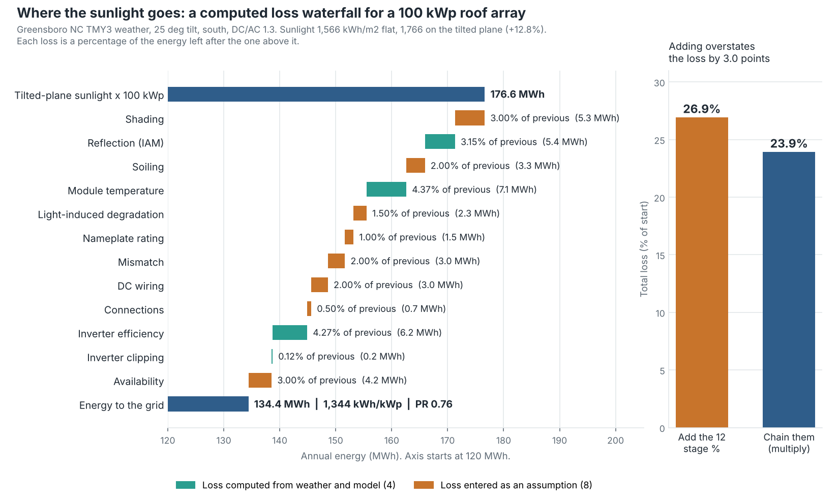
Figure 1. Twelve losses take a 100 kWp array from 176.6 to 134.4 MWh, and adding their percentages overstates the loss by 3.0 points.
Do you add or multiply loss percentages?
Multiply when each loss is a percentage of the energy left. Add only when every percentage is of the same starting energy. Mixing the two is the most common maths slip.
Take a 10% loss then a 5% loss on 1,000 kWh. The first leaves 900 kWh. The second takes 45 kWh of that, so the total is 14.5%, not 15%. Aurora’s help gives the same rule: losses of 4% and 3% combine to 6.88%. SAM and pvlib document the same product form.
- Sample result: the 12 stage percentages add to 26.9%. Chained, they give 23.9%. Adding would predict 129,112 kWh instead of 134,411, which is 3.9% too low.
- Published report: net of its one gain, the 22 percentages after the irradiance gain add to 16.1%. Chained they give 15.0%.
- Order: the total does not change if you reorder stages. Each line’s kWh does. Our 3% availability loss removes 4.2 MWh in last place and 5.3 MWh if it came first.
- Same basis: expressed as a percentage of the start, our 12 losses do add, to 23.9%.
Worked example: a 100 kWp roof array
We built the waterfall in pvlib 0.16.1 on one weather file. The table shows each stage, how it was set, and the energy left.
System: 100 kWp, fixed tilt 25 degrees, facing south, DC/AC ratio 1.3 (76.9 kW AC). Weather: the Greensboro, North Carolina TMY3 file that ships with pvlib. Sunlight: 1,566 kWh/m² flat and 1,766 on the tilted plane, using the Perez model and albedo 0.2. Cell temperature: SAPM open-rack glass-glass model with a -0.35%/K coefficient, which is our choice.
| Loss | How set | % of previous | Energy left (kWh) |
|---|---|---|---|
| Start: tilted-plane sunlight × 100 kWp | Computed | - | 176,634 |
| Shading | Assumed 3% (PVWatts default) | 3.00% | 171,335 |
| Reflection (IAM) | Computed: pvlib physical IAM model | 3.15% | 165,946 |
| Soiling | Assumed 2% (PVWatts default) | 2.00% | 162,627 |
| Module temperature | Computed: cell temperature, -0.35%/K | 4.37% | 155,517 |
| Light-induced degradation | Assumed 1.5% (PVWatts default) | 1.50% | 153,184 |
| Nameplate rating | Assumed 1% (PVWatts default) | 1.00% | 151,652 |
| Mismatch | Assumed 2% (PVWatts default) | 2.00% | 148,619 |
| DC wiring | Assumed 2% (PVWatts default) | 2.00% | 145,647 |
| Connections | Assumed 0.5% (PVWatts default) | 0.50% | 144,918 |
| Inverter efficiency | Computed: PVWatts curve, 96% nominal | 4.27% | 138,733 |
| Inverter clipping | Computed: AC cap at 76.9 kW | 0.12% | 138,569 |
| Availability | Assumed 3% (PVWatts default) | 3.00% | 134,411 |
| Energy to the grid | Chained | 23.90% total | 134,411 |
The result is 1,344 kWh/kWp and a performance ratio of 0.761. That differs from the 84.1% on our performance ratio page. It is a different system with different losses. See performance ratio for what that number means.
As a share of the starting energy, the groups are irradiance 7.9%, temperature 4.0%, DC 6.0%, inverter 3.6% and availability 2.4%. They add to 23.9%.
Eight of the 12 losses are PVWatts defaults, taken as pvlib documents them, so the sample has limits. Our inverter uses the generic 96% nominal efficiency, so its line is bigger than the PVsyst report’s. The sample has no AC cable or transformer line. A pvlib ModelChain run on the same weather and the same ten loss defaults gives 1.3% more AC energy (136,166 kWh). It has 0.9% less sunlight on the plane (1,751 against 1,766 kWh/m²). The two model chains differ in ways we did not test, so the gap is unexplained. Treat our 23.9% as a teaching figure, not a validated one.
Loss chain calculator
Enter your own stage percentages to compare the chained total with the added total. The loss chain calculator also opens on its own page, which suits a phone.
How solar software handles the loss diagram
All six tools we checked draw or compute a loss chain, but only some state the basis of each percentage. The table covers only what each company’s own documentation says, checked October 2026.
| Software | Does it show a loss diagram? | Where to find it | Notes |
|---|---|---|---|
| PVsyst | Yes | Simulation report, full year. Monthly under Detailed results | Each loss is a percentage of the previous energy quantity. |
| SAM | Yes | Losses tab on the Results page, drawn as a Sankey diagram | SAM’s help says it is not shown for all performance models. |
| HelioScope | Yes | Sources of System Loss chart and Annual Production table | A wheel-style chart, not a waterfall. Losses are multiplicative. A white gap marks a gain. |
| Aurora Solar | Yes | Simulation panel, Advanced menu, after a performance simulation | Article updated 13 May 2026. Separate System Losses page says losses are multiplicative. |
| Solargis Evaluate | Yes | Loss table in its knowledge base | Three bases per step. Its overview page (updated 24 September 2026) also mentions a simple-sum option without reconciling it. |
| pvlib python | Partly | pvlib.pvsystem.pvwatts_losses | Combines the ten PVWatts loss inputs by product. It draws no diagram. |
Partly: the tool combines losses but draws no diagram. For more tools that model losses, see the best solar design software.
Common mistakes with loss diagrams
FAQs
What is a normal total system loss?
There is no single normal figure. HelioScope’s Loss Factors page lists a typical total performance ratio of 68% to 88%, but it says that ratio excludes the plane-of-array irradiance step. So do not read one minus that ratio as the total loss. Our sample loses 23.9% on one unvalidated model run, and the PVsyst report we checked shows a ratio of 0.852.
Is a loss diagram the same as performance ratio?
No. The diagram splits the loss by cause. Performance ratio is one number for the whole chain. HelioScope notes that its performance ratio total excludes the plane-of-array irradiance step.
Why does my diagram not add up?
Each percentage is usually of the previous step, so adding them gives the wrong total. Rounding and hidden gains also matter. Our PVsyst check had one +0.50% gain, and it matched once chained.
Which losses can a designer change?
Layout and equipment choices change shading, mismatch, wiring and the DC/AC ratio. Mounting style changes temperature, and HelioScope’s range is wider for flush mounts. Availability depends on maintenance and the grid.
What does a gain on the diagram mean?
A step that adds energy shows as a gain. Tilting the plane is one. PVsyst’s module quality line was +0.50% in the report we checked. HelioScope shows gains as a white gap in its chart.
Related terms
- Performance ratio: the whole chain as one number.
- Energy yield simulation: the hourly run that produces the diagram.
- Mismatch loss: one line of the diagram, covered in depth.
Next step: to compare how simulation tools draw their loss diagrams, read the best solar simulation software list.
Sources
- PVsyst help: loss diagram. Array and system losses (checked October 2026).
- PVsyst V7.4.5 simulation report for a 52.62 MWp UK site, dated 4 March 2024. It is a public planning document (checked October 2026).
- Aurora help: System Loss Diagram (updated 13 May 2026). System Losses (dated 29 June 2026, checked October 2026).
- HelioScope help: Loss Factors. How to Troubleshoot Losses (no date shown in the text we read, checked October 2026).
- SAM help: loss diagram. PV losses (checked October 2026). SAM’s help is hosted on nlr.gov because the US Department of Energy renamed the National Renewable Energy Laboratory to the National Laboratory of the Rockies (NLR) in December 2025. Its pages now credit both names.
- Solargis knowledge base: PV system losses (last updated 24 September 2026). Losses in detail (checked October 2026).
- pvlib documentation: pvwatts_losses. Inverter.pvwatts (checked October 2026).
- Dobos, Freeman and Blair, Improvements to PVWatts for Fixed and One-Axis Tracking Systems, NREL/CP-6A20-74097, June 2019. Its loss diagram percentages are relative to the previous energy value and not additive. The old nrel.gov link now redirects to nlr.gov (checked November 2026).
Last updated 30 October 2026. Next scheduled review: 30 January 2027.