Key takeaways
- A solar model has five blocks, from inputs to outputs. The FAST Standard asks for separate sheets by type: foundation, workings, presentation and control.
- This example’s 2 MWdc project has capex of 2.30 million USD and debt of 1.51 million USD. Project IRR is 6.77%, equity IRR is 8.42% and the lowest debt cover is 1.30.
- Moving price or yield by 10% shifted equity IRR by about 2.2 to 2.4 points. Degradation moved it by 0.10 points.
- A combined downside (P90 energy, flat price, O&M up 10%) took equity IRR to 2.12% and lowest debt cover to 0.92. Six years fell below 1.00.
- Six seeded mistakes moved equity IRR by 0.13 to 4.78 points. A targeted check flagged each one, but "NPV at the IRR is zero" flagged none.
To build debt, tax and what-if cases in software, see the best solar financial modelling software.
Financial modelling at a glance
A financial model is a set of linked calculations. It answers "what do we earn, and how sure are we?" for one set of assumptions.
| Item | Detail |
|---|---|
| Core chain | Size × yield × availability × degradation = energy. Energy × price = revenue. Revenue − costs = EBITDA. EBITDA − debt service − tax = cash to equity. |
| Outputs | Cash flow, IRR, NPV, payback, LCOE and debt cover. Our example: 8.42% equity IRR, 1.30 lowest cover. |
| Where it matters | Commercial and utility proposals, lender and investor packs, PPA pricing, go or no-go studies. |
| Standard or rule | No solar-specific standard was found. The FAST Standard (July 2019) sets rules for how to build a spreadsheet, such as consistent formulas and no embedded constants. |
| In software | Design and finance tools bundle a financial block. Depth of debt, tax and what-if tools differs. |
Why does financial modelling matter for installers?
The model sets the price a buyer sees and the debt a lender offers. Small slips can hide inside a model that still gives a tidy IRR.
In the seeded-mistake table below, one wrong O&M unit lifted equity IRR by 4.78 points. A buyer’s finance team will ask what sits behind the headline number. You need a structure you can explain. You also need checks you can show. For the cash flow table itself, see cash flow analysis.
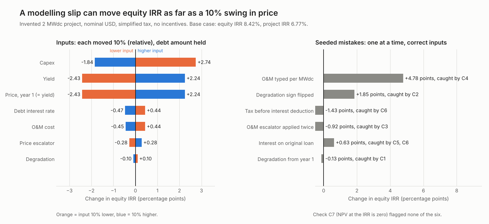
Figure 1. A single modelling slip can move equity IRR as far as a 10% swing in price. Only targeted checks flag it.
What are the blocks of a solar financial model?
A solar model has five blocks. Inputs feed a yield-to-revenue chain, a cost block and a debt and tax block. Outputs read from all of them.
- Inputs. Size, capex, yield, availability, degradation, price, escalators, O&M, debt terms and tax. Each input has one cell and one unit.
- Yield-to-revenue chain. Energy comes from an energy yield simulation, less degradation. Price turns energy into revenue. See power purchase agreements.
- Costs. Year-0 capex, then yearly O&M and other opex.
- Debt and tax. A loan schedule gives interest and principal. Tax uses profit after depreciation and interest.
- Outputs. Cash flow, IRR, NPV, payback and debt cover, plus the audit checks.
The FAST Standard (version 02c, July 2019) gives related rules for sheets. Quotes are as printed in the PDF on fast-standard.org.
- Rule 1.01-01: "Separate worksheets by type: Foundation, Workings, Presentation and Control."
- Rule 3.02-01: "Formulas must be consistent".
- Rule 3.04-01: "Do not write formulas with embedded constants".
- Rule 3.05-04: "Include a units designator on all line items".
- Rule 2.03-05: "Include master error checks and alert indicators in the freeze pane".
HelioScope’s help shows the same idea in a tool. In a project, you can set its financial inputs as editable or locked (help article dated 4 September 2026 as it prints).
Worked example: a 2 MWdc commercial project
Year 1 of our example turns 2.97 million kWh into 48,104 USD of cash to equity. The figures are computed in code, and the calculator gives the same results. This example project differs from the one on the IRR page.
| Input (example) | Value |
|---|---|
| Size and capex | 2,000 kWdc at 1.15 USD per W = 2,300,000 USD at year 0 |
| Energy | 1,500 kWh per kWdc (P50 yield) × 99% availability. Degradation 0.5% a year from year 2. 25 years |
| Price | 0.085 USD per kWh in year 1, rising 1.5% a year |
| O&M | 22 USD per kWdc in year 1 (44,000 USD), rising 2% a year |
| Debt | Sized so the lowest year of EBITDA ÷ debt service is 1.30. Capped at 70% of capex. 6.5%. 15 level payments |
| Tax | Flat 25% of EBITDA − depreciation − interest, floored at zero. Straight-line depreciation over 20 years. No loss carry-forward |
| Left out | Incentives, reserve accounts, fees, land, insurance and working capital |
| Year-1 line | Value | How it is built |
|---|---|---|
| Energy | 2,970,000 kWh | 2,000 × 1,500 × 0.99 |
| Revenue | 252,450 USD | Energy × 0.085 |
| O&M | 44,000 USD | 2,000 × 22 |
| EBITDA | 208,450 USD | Revenue − O&M |
| Debt service | 160,346 USD | 1,507,682 USD at 6.5% over 15 years, level payments |
| Tax | 0 USD | 208,450 − 115,000 depreciation − 97,999 interest is below zero |
| Cash to equity | 48,104 USD | EBITDA − debt service − tax |
Debt is 65.6% of capex, so equity puts in 792,318 USD at year 0. Project IRR is 6.77% and equity IRR is 8.42%. The lowest debt cover is 1.30 by design. The average is 1.37. Energy in year 25 is 2,633,361 kWh, which is 11.3% below year 1. We measure debt cover on pre-tax EBITDA. That avoids a loop between tax and debt. Lenders set their own cover terms. For what IRR and NPV mean, see the IRR and NPV pages.
How should you test a model: sensitivity or scenarios?
Sensitivity moves one input at a time. A scenario moves several inputs together under a name. Use sensitivity to find what matters. Use scenarios to test what could go wrong at once.
Our sensitivity moves each input 10% (relative). The debt amount stays at 1,507,682 USD. A real loan does not shrink when yield falls. Capex and yield or price move equity IRR the most.
| Input moved 10% | Equity IRR change, points (lower / higher) |
|---|---|
| Capex | +2.74 / −1.84 |
| Yield, or price in year 1 | −2.43 / +2.24 |
| Debt interest rate | +0.44 / −0.47 |
| O&M | +0.44 / −0.45 |
| Price escalator | −0.28 / +0.28 |
| Degradation | +0.10 / −0.10 |
Yield and price share one row because they move revenue in the same way. A 10% move in a 0.5% degradation rate is only 0.05 points of rate. Equal relative moves are not equally likely, so pick each range from evidence. Yield or price at minus 10% also cut lowest debt cover from 1.30 to 1.14.
The next table shows how combined downsides hit returns and debt cover. Scenarios keep the debt amount at the base figure too, unless the row says "re-sized". Our P90 factor is 0.8975. We get it from P90 = P50 × (1 − 1.2816 × U) with an example U of 8%. See P50, P90 and P99.
| Scenario (debt held unless stated) | Equity IRR | Project IRR | Lowest cover | Years below 1.00 |
|---|---|---|---|---|
| Base (P50) | 8.42% | 6.77% | 1.30 | 0 |
| P90 energy only | 5.93% | 5.55% | 1.14 | 0 |
| Flat price (0% escalator) only | 5.44% | 5.17% | 1.11 | 0 |
| O&M up 10% only | 7.98% | 6.55% | 1.27 | 0 |
| Combined downside | 2.12% | 3.63% | 0.92 | 6 |
| Combined downside, debt re-sized to 1.30 (1,065,754 USD) | 2.95% | 3.63% | 1.30 | 0 |
The three single effects sum to −5.92 points. The combined case is −6.31. Effects interact, so adding single tests understates a joint downside. Re-sizing debt raised equity IRR here only because debt at 6.5% costs more than the project’s 3.63% return. In the combined row, a year where debt service is above EBITDA counts as an equity top-up.
Which checks catch model errors?
Each check should test one thing the model could get wrong, from outside the formula chain. Six mistakes were put into the correct model, one at a time, and seven checks were run. The table shows which check flagged which mistake.
| Check | Test | Seeded mistake it flagged (equity IRR change) |
|---|---|---|
| C1 | Year-1 energy equals size × yield × availability | Degradation applied from year 1 (−0.13 points) |
| C2 | Energy never rises when degradation is above zero | Degradation sign flipped (+1.85) |
| C3 | O&M path matches an independent formula | O&M escalator applied twice (−0.92) |
| C4 | O&M input sits inside a sanity band (this example’s band: 5 to 60 USD per kWdc per year) | O&M typed per MWdc, so 1,000 times too small (+4.78) |
| C5 | Loan balance is zero after the last payment | Interest charged on the original loan (+0.63) |
| C6 | Tax equals rate × (EBITDA − depreciation − interest) | Tax before the interest deduction (−1.43) |
| C7 | NPV at the reported equity IRR is zero | None of the six |
C7 passes every time because it tests the solver, not the logic. A passing check proves only what it tests. Only one check caught the smallest slip, 0.13 points. It was C1.
These checks are our design. They match the spirit of FAST Appendix B: a check "should not fail" whatever the scenario. Run them on every scenario, not only the base case. Set a band like C4 from your own past projects, because ours is example.
Solar financial model checker
The presets match the tables above. The seed menu matches the audit table. The calculator warns about blank, zero, negative or out-of-range inputs instead of showing a wrong number. It is a design aid, not financial advice.
How solar software handles financial modelling
All five tools below name a tax input. They differ on debt and on what-if tools: only SAM lists parametric and stochastic runs, and Aurora’s loan inputs cover customer payments. The pages were checked October 2026.
| Software | Debt and tax inputs | What-if tools | Source and date |
|---|---|---|---|
| SAM | Debt: yes. Tax: yes. | Yes: parametrics and stochastic runs | SAM help, financial parameters and simulation options. No date shown. Twelve financial models listed |
| Solargis Prospect | Debt: yes. Tax: yes. | Partly: saved input sets | Solargis knowledge base, updated 24 September 2026 |
| HelioScope | Debt: Not stated. Tax: yes, effective tax rate and depreciation. | Partly: yearly debug view | Depreciation article updated 8 July 2025. Debug article: no date shown. Step-by-step article dated 4 September 2026 |
| Aurora Solar | Debt: partly, customer loan rate, dealer fee and term. Tax: yes, rates and depreciation (MACRS, straight-line or none). | Partly: with and without solar | Aurora help, updated 15 May 2026 |
| PVsyst | Debt: yes, the Loans input. Tax: yes, the “Income tax rate” input. | Not stated | PVsyst help, financial parameters and economic evaluation. No date shown |
"Yes" means the page names the input or tool. "Partly" means it names a narrower input than the full job. "Not stated" means the pages read do not mention it. That covers the HelioScope debt input and PVsyst what-if tools. PVsyst batch and parametric pages were not among the pages read. For tools that build debt, tax and what-if cases, see the best solar financial modelling software.
Common mistakes with financial modelling
FAQs
What is the difference between sensitivity and scenario analysis?
Sensitivity changes one input and holds the rest. Scenario analysis changes several inputs together, such as P90 energy, flat price and higher O&M. In our example the three single effects summed to −5.92 points. The combined case gave −6.31.
What should a solar financial model include?
A solar financial model turns energy yield into cash flow, IRR, NPV, payback and debt cover. It should include five blocks: inputs, a yield-to-revenue chain, costs, debt and tax, and outputs. Keep sheets separate by type, as the FAST Standard asks. Add audit checks and test more than one scenario, so the results show a range.
Should debt be re-sized when I test a downside?
Do both, and label which is which. Hold the loan amount to see whether the project can pay the debt it has. Re-size to see what a lender might offer on that case. Annual debt service equals the lowest EBITDA divided by the target cover. Our combined downside gave debt cover of 0.92 when held. It gave 1.30 when re-sized to 1,065,754 USD.
How do I check a solar financial model for errors?
Test inputs, schedules and logic separately. Tie year-1 energy back to size and yield. Check that the loan reaches zero. Work out tax again from its parts. Add range bands on inputs. Run every check on every scenario.
Does a financial model predict returns?
No. It shows what follows from your assumptions. So show the range and state each assumption beside each result. For real versus nominal rates, see NPV.
Why do two tools give different results for one project?
Often the blocks differ: tax, debt, timing, horizon or incentives. In our example, one modelling choice alone moved the combined downside from 2.12% equity IRR with debt held to 2.95% when re-sized.
Related terms
- Cash flow analysis: the year-by-year table the model builds.
- Feasibility study: an early check of whether a project is worth modelling in full.
- IRR and NPV: the two return measures the model reports.
Next step: compare how tools handle debt, tax and what-if cases in the best solar financial modelling software.
Sources
- FAST Standard 02c, July 2019, official PDF on fast-standard.org. Rule quotes read there (checked 30 October 2026). A copy is also hosted by STL Training.
- Solargis knowledge base: Financial analysis, updated 24 September 2026 (checked October 2026).
- HelioScope: How to Model Depreciation, updated 8 July 2025 (checked October 2026).
- HelioScope: Step-by-Step Guide, Creating a Financial Model, dated 4 September 2026 as it prints (checked October 2026).
- HelioScope: Accessing the Financial Debug Feature, no date shown (checked October 2026).
- Aurora help: Financial analysis overview, updated 15 May 2026 (checked October 2026).
- SAM help: Financial parameters and simulation options, no date shown (checked October 2026).
- PVsyst help: financial parameters and economic evaluation, no date shown (checked October 2026).
Last updated 30 October 2026. Next scheduled review: 30 January 2027.