Key takeaways
- This example’s 100 kWdc rooftop (160,000 USD capex, nominal, pre-tax) has cumulative cash of 407,556 USD at year 25.
- At a 6% discount rate, the same table gives an NPV of 114,001 USD.
- Net cost divided by year-1 net cash gives 8.8 years. The full table gives 8.2, because savings rise.
- Repeating year-1 net cash for 25 years ends 115,056 USD below the table (292,500 USD against 407,556 USD).
- With a 70% loan at 7% over 10 years, net cash in year 1 is only 2,154 USD. Cumulative cash turns positive at 10.4 years.
To model your own cash flow with debt and tax, see the best solar financial modelling software.
Cash flow analysis at a glance
A cash flow table lists every amount in and out for each year. Payback, NPV and IRR are all read from it.
| Item | Detail |
|---|---|
| Net cash formula | Net cash in year t = savings or revenue − O&M − one-off costs + incentives − loan payments. |
| Cumulative formula | Cumulative cash = the running total of net cash from year 0. |
| Unit and range | USD per year, nominal unless the table says real. Our example: 18,100 USD net in year 1, 28,720 USD in year 25. |
| Where it matters | Commercial proposals, lender and investor packs, and the cash flow chart a salesperson shows a buyer. |
| Standard or rule | No single standard. Tools differ on start year, end year, tax and what counts as a flow. |
| In software | Proposal, design and finance tools show an annual table or chart. Some also show a cumulative line. |
Why does cash flow analysis matter for installers?
It shows when the buyer is ahead and how much they hold at each stage. A single payback number hides the dip from a replacement or a loan.
The same table feeds payback period, NPV and IRR. If your inputs are wrong here, all three are wrong. Aurora’s help says the annual view shows each year’s net result as a bar.
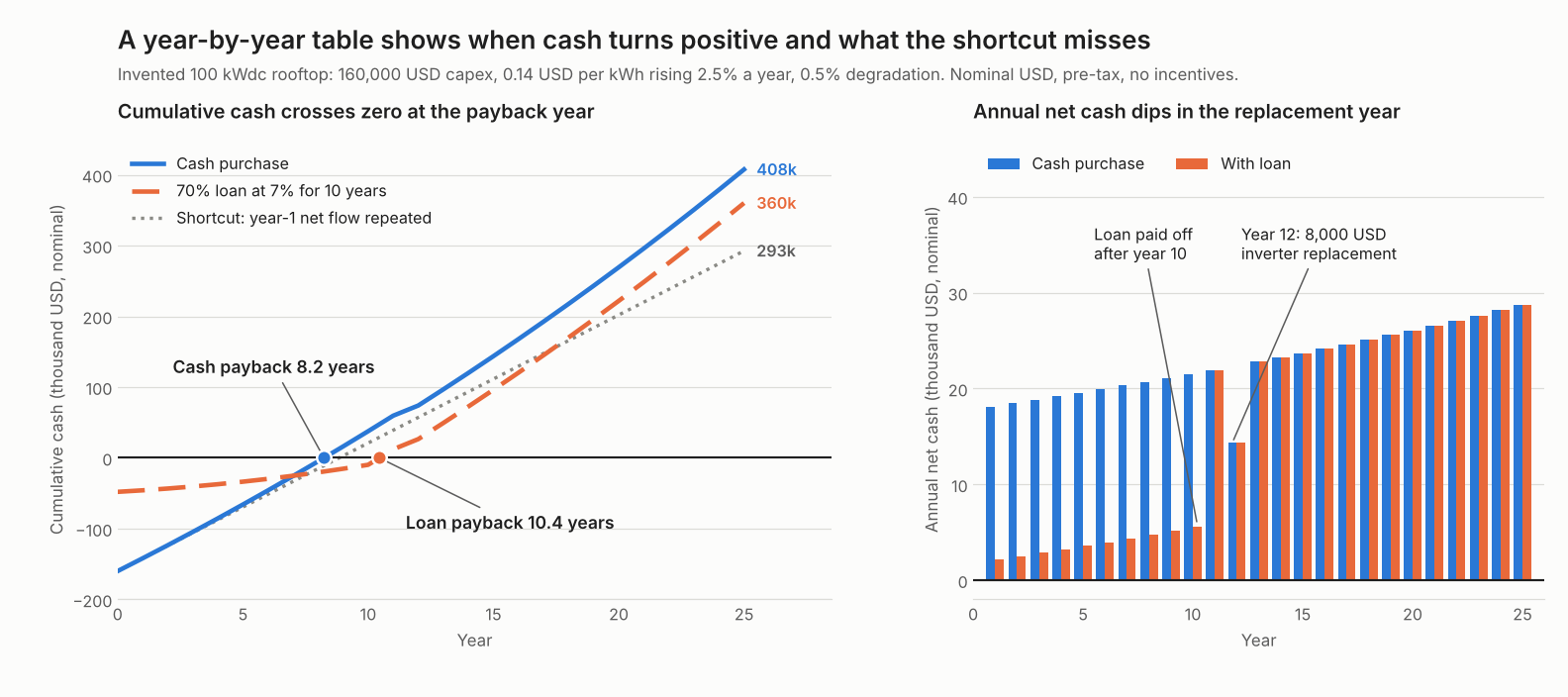
Figure 1. In our example case, cumulative cash turns positive at 8.2 years for cash and 10.4 with a loan. The year-1 shortcut ends 115,056 USD lower.
How do you build a cash flow table?
Start with year 0 as the outlay, then add one row per year. Each row is savings less costs, plus or minus one-off items.
- Fix the convention and write it above the table. State the outlay at year 0, flows at year end, nominal or real, and tax in or out.
- Take year-1 energy from a yield simulation. Scale later years by degradation: kWh in year t = year-1 kWh × (1 − d)^(t − 1). See degradation rate.
- Value each kWh. For savings, use the customer’s tariff (see tariff databases and net metering). For sales, use the PPA price. Raise it by the escalation rate.
- Subtract O&M and any one-off cost, such as an inverter replacement. Add an incentive in the year it is received.
- If financed, reduce the year-0 outlay by the loan. Subtract the level loan payment in each loan year.
- Add the lines to get net cash. Keep a running total for cumulative cash. Divide each net by (1 + r)^t and total those for discounted cash.
Payback is where the cumulative line crosses zero, found by interpolation inside that year. The last discounted total equals NPV. For the cost lines, see CAPEX and OPEX.
Worked example: a 100 kWdc rooftop, cash and loan
This example’s rooftop has capex of 160,000 USD. It turns cumulative cash positive at 8.2 years on a cash purchase. The calculator below reproduces every figure.
| Input (example) | Value |
|---|---|
| Size and capex | 100 kWdc at 1.60 USD per W = 160,000 USD at year 0 |
| Energy | 1,400 kWh per kWdc in year 1 (140,000 kWh), falling 0.5% a year. 25 years |
| Value of energy | 0.14 USD per kWh in year 1, rising 2.5% a year |
| O&M | 15 USD per kWdc in year 1 (1,500 USD), rising 2.5% a year |
| Inverter replacement | 0.08 USD per W (8,000 USD) in year 12, not escalated |
| Loan case | 70% of capex (112,000 USD) at 7% over 10 years. Level payment 15,946 USD |
| Discount rate | 6% nominal, for the discounted column only |
| Left out | Tax, depreciation, incentives (except the test below), fees, insurance and land |
The first table below shows the inputs for one cash purchase in selected years. The second shows the running cash. Amounts are in USD, rounded, so a row can differ by 1 USD. Costs are shown as positive amounts. The year-12 figure is the inverter replacement.
| Year | Energy (kWh) | Savings | O&M | Other costs |
|---|---|---|---|---|
| 0 | - | - | - | - |
| 1 | 140,000 | 19,600 | 1,500 | 0 |
| 5 | 137,221 | 21,205 | 1,656 | 0 |
| 8 | 135,173 | 22,495 | 1,783 | 0 |
| 9 | 134,497 | 22,942 | 1,828 | 0 |
| 12 | 132,490 | 24,337 | 1,968 | 8,000 |
| 13 | 131,827 | 24,821 | 2,017 | 0 |
| 25 | 124,131 | 31,433 | 2,713 | 0 |
| Year | Net cash | Cumulative | Discounted cumulative |
|---|---|---|---|
| 0 | -160,000 | -160,000 | -160,000 |
| 1 | 18,100 | -141,900 | -142,925 |
| 5 | 19,550 | -65,911 | -80,910 |
| 8 | 20,712 | -4,952 | -40,353 |
| 9 | 21,114 | 16,162 | -27,856 |
| 12 | 14,369 | 73,999 | 2,864 |
| 13 | 22,804 | 96,803 | 13,555 |
| 25 | 28,720 | 407,556 | 114,001 |
Cumulative cash crosses zero between years 8 and 9: 8 + 4,952 ÷ 21,114 = 8.2 years. Discounted at 6%, it crosses in year 12 (11.6 years by interpolation). The year-25 discounted total, 114,001 USD, is the NPV.
Loan case, same inputs. Year 0 is the 48,000 USD equity outlay (160,000 less 112,000).
| Year | Loan payment | Net cash | Cumulative |
|---|---|---|---|
| 0 | +112,000 received | -48,000 | -48,000 |
| 1 | -15,946 | 2,154 | -45,846 |
| 5 | -15,946 | 3,603 | -33,642 |
| 10 | -15,946 | 5,578 | -9,776 |
| 11 | 0 | 21,943 | 12,167 |
| 25 | 0 | 28,720 | 360,093 |
The loan cuts the outlay from 160,000 to 48,000 USD. It also leaves a thin cushion in years 1 to 10, and payback moves to 10.4 years. It ends 47,463 USD lower, the interest paid (159,463 over 10 years less 112,000 principal).
One input at a time, with the rest at base, for the cash purchase. The test ranges differ in size, so this is not a ranking.
| Input changed | Test value | Payback (years) | Cumulative at year 25 (USD) |
|---|---|---|---|
| Value escalation | 0% a year | 9.1 | 242,460 |
| Value escalation | 5% a year | 7.6 | 651,271 |
| Value, year 1 | 0.12 USD per kWh | 9.6 | 318,014 |
| Value, year 1 | 0.16 USD per kWh | 7.2 | 497,098 |
| Capex | 1.40 USD per W | 7.3 | 427,556 |
| Capex | 1.80 USD per W | 9.2 | 387,556 |
The next table covers running costs, degradation and the inverter replacement.
| Input changed | Test value | Payback (years) | Cumulative at year 25 (USD) |
|---|---|---|---|
| O&M, year 1 | 10 USD per kWdc | 8.0 | 424,635 |
| O&M, year 1 | 25 USD per kWdc | 8.7 | 373,398 |
| Degradation | 0.3% a year | 8.2 | 424,225 |
| Degradation | 0.8% a year | 8.3 | 383,534 |
| Inverter replacement, year 12 | none | 8.2 | 415,556 |
| Inverter replacement, year 12 | 0.16 USD per W | 8.2 | 399,556 |
The replacement does not move payback because it falls after payback. Put the same 0.16 USD per W in year 6 and payback moves to 9.0 years. Timing matters as much as size.
Calculator: build your own cash flow table
Enter your inputs to print the full yearly table, payback and NPV. The defaults are the example above.
How do tax and incentives enter the table?
Tax and incentives add lines to the table, and each tool treats them differently. Our example has no tax, so it is a pre-tax view only. We state no solar tax rule here. Ask a tax adviser and check the date of any rule you rely on.
Aurora’s help says commercial tax rates are required for depreciation calculations and for the after-tax value of savings and incentives. It adds that incentive payments are applied in the year they are received. Year-0 cash grants reduce the starting net cost. Solargis Prospect lists "Taxes on profit" and "Linear tax depreciation" as inputs.
Incentive timing changes the table even when the amount is fixed. A placeholder 48,000 USD incentive (30% of capex, our number, not a rule) shows the effect. Paid in year 0 it cuts the lowest cumulative cash from -160,000 to -112,000 USD. Paid in year 0, 1 or 2, payback stays at 5.9 years. NPV is 162,001, 159,284 and 156,721 USD.
How solar software handles cash flow analysis
All six tools we checked print a yearly table, and only Aurora, PVsyst and HOMER Front also show a cumulative line. Checked October 2026.
| Software | Year-by-year cash flow? | Cumulative cash? | Source |
|---|---|---|---|
| Aurora Solar | Yes | Yes | Aurora help, no update date shown |
| HelioScope | Yes | Not stated | HelioScope help, no date shown |
| PVsyst | Yes | Yes | PVsyst help, undated |
| HOMER Front | Yes | Yes | HOMER help, updated 19 October 2026 |
| Solargis Prospect | Yes | Not stated | Solargis knowledge base, updated 24 September 2026 |
| SAM | Yes | Not stated | SAM help, undated |
Not stated means the company page we cite does not say. Here is what each page says.
- Aurora Solar: Cash flow chart in Sales Mode with annual and cumulative views. Lists incentives, loan payments, degradation, O&M with inverter replacement (commercial only) and rate escalation. Its help says the cashflow table runs to year 24, while lifetime savings cover the full 25-year project life.
- HelioScope: Cash Flow Table tracks bill savings, incentives, operating expenses and debt payments by period.
- PVsyst: "the annual balance as well as the accumulated balance" over the lifetime, with an annual table.
- HOMER Front: Cash flow view with revenue, operating expenses, net operating income and cumulative cash flow, which includes replacement costs. The help page is in the HOMER Front manual.
- Solargis Prospect: Cash Flow table with yearly Revenue and OPEX columns. A cumulative total appears only on an energy column.
- SAM: "The Cash flow tab displays the project cash flow calculated by the financial model." Exports CSV and Excel.
For ranked tools, see the best solar financial modelling software and the best solar proposal software.
Common mistakes with cash flow analysis
FAQs
What is the difference between cash flow analysis and NPV?
Cash flow analysis is the yearly table. NPV is one figure taken from it. Divide each year’s net cash by (1 + r)^t, then add the year-0 outlay. In our example the year-25 discounted total, 114,001 USD, is the NPV. See the NPV page.
How do you read a cumulative cash flow chart?
The line starts negative at year 0. Aurora’s help says the breakeven point is "The year the cumulative line crosses zero". Our cash case crosses at 8.2 years and then rises to 407,556 USD at year 25.
Why does the chart payback differ from the payback metric?
The cumulative chart crosses zero at 8.2 years because savings rise each year. Net cost divided by year-1 net cash gives 8.8 years in our example. A payback metric that divides by one year of savings, as Aurora’s help describes, will not always match the chart. Discounted at 6%, our payback is 11.6 years.
Does a cash flow table include tax?
Only if the tool or the analyst adds it. Aurora needs tax rates for commercial depreciation and after-tax value. Our example is pre-tax. Always label the table.
Related terms
- NPV: the year-0 outlay plus discounted net cash.
- IRR: the discount rate at which NPV is zero.
- Payback period: recovery time.
- Feasibility study: the wider review.
- Debt sizing and DSCR: how much debt a project cash flow can repay.
Next step: run your own project through a tool from the best solar financial modelling software list and compare its table with ours.
Sources
- Aurora help: Financial analysis overview, no update date shown (checked 30 October 2026).
- HelioScope help: Cash Flow Table, no date shown (checked 30 October 2026).
- PVsyst help: financial results, undated (checked 30 October 2026).
- HOMER help: cash flow view, updated 19 October 2026 (checked 30 October 2026).
- Solargis knowledge base: Financial analysis, updated 24 September 2026 (checked 30 October 2026).
- SAM help: Cash flow, undated (checked 30 October 2026).
Last updated 30 October 2026. Next scheduled review: 30 January 2027.