Key takeaways
- Our example (9,000 kWh, 0.20 USD per kWh, 0.5% degradation) saves 54,045 USD over 25 years with a 2% yearly rise. It saves 69,924 USD with 4% and 42,401 USD with 0%.
- The rise must beat degradation to lift yearly savings. In the example, a rise of about 0.50% almost exactly cancels 0.5% degradation (exact break-even 0.5025%).
- EIA’s US average residential price grew 0.8% a year in 2015 to 2020 and 5.6% in 2020 to 2025 (nominal). The window you pick sets the rate.
- Prices do not rise every year. Two of 15 yearly changes from 2010 to 2025 were falls. California’s 2025 residential average was below 2024 (EIA).
Escalation is a named input in proposal tools, and the best solar proposal software list covers them.
Utility rate escalation at a glance
It answers one question: how fast will the power price that solar avoids rise? You choose the number, so it is an assumption and not a measured fact.
| Item | Detail |
|---|---|
| Formula | Price in year t = year-1 price × (1 + e)^(t − 1), where e is the escalation rate as a decimal. |
| Unit and range | Percent a year, nominal unless the tool says real. This example’s cases are 0%, 2% and 4%. EIA’s US residential history gives 0.8% to 5.6% a year, depending on the window. |
| Where it matters | Bill savings in proposals, and every long-horizon output built on them: payback, NPV, IRR and ROI. |
| Standard or rule | No standard found. The tools below each set their own default and basis. |
| In software | A named input in proposal and financial tools. See the software table. |
Why does the escalation rate matter for installers?
It grows the saving in every later year, so it moves each long-run result. Two quotes for one roof can differ only in this input.
Aurora’s help lists the utility escalation rate as a key driver of bill savings. It says a "higher escalation rate increases projected savings". A rep who cannot name the rate in a quote cannot defend the savings. For the full set of outputs, see financial modelling. The payback, NPV, IRR and ROI pages test the rate on their own example homes. This page shows how to pick and check it.
How does utility rate escalation differ from a contract escalator, degradation and the discount rate?
They are four separate numbers. Utility escalation raises the price you avoid, and a contract escalator raises what the host pays. Degradation cuts output, while the discount rate cuts the value of later cash.
| Number | Whose number it is | What it changes | Where tools set it |
|---|---|---|---|
| Utility rate escalation | Your assumption about the tariff | Price per kWh avoided, rising | Aurora: Settings > Utility and tax rates. HelioScope: Financial Templates, Modeling. |
| Contract escalator | Set in a lease or PPA contract | The payment or price per kWh the host pays the owner | Lease and PPA inputs. See solar lease and power purchase agreement. |
| Degradation | Module ageing, see degradation rate | kWh produced, falling | HelioScope: Annual Degradation Rate. Aurora: Advanced financing settings. |
| Discount rate | The owner’s time value of money | Present value of every cash flow | Aurora: Settings > Financing. HelioScope: Financing. |
Under a lease or PPA both act. The host’s saving in year t is the bill avoided that year minus that year’s payment. The third-party ownership page tests that pair.
The rise and the discount rate pull in opposite directions. With no degradation, equal rates give every year’s saving the same present value. At 5% for both, each year of our example is worth 1,714 USD. So 25 years total 42,857 USD. Keep the basis matched. A nominal rise needs a nominal discount rate, as the NPV page explains.
How do you apply utility rate escalation in a savings model?
Grow the price by (1 + e) each year. Shrink the output by (1 − d). Then multiply. The saving in year t is that year’s output times its price.
- Set the year-1 price from the customer’s tariff. See tariff rate databases and bill offset.
- Pick e. Write beside it whether it is nominal or real.
- Output in year t = year-1 output × (1 − d)^(t − 1), with d the degradation rate.
- Saving in year t = output × year-1 price × (1 + e)^(t − 1). Value exports apart if the tariff differs.
- Add the yearly savings for the total. For present value, divide each by (1 + r)^t, with r the discount rate.
- Check the yearly change in saving: (1 + e)(1 − d) − 1. It is zero when e = d ÷ (1 − d).
A tool may not do exactly this. Aurora’s help says it calculates bill savings with an hourly simulation. So the rate acts on a modelled bill.
What does the price history say about the escalation rate?
History gives a wide range. EIA’s US average residential price rose from 8.24 cents per kWh in 2000 to 17.30 in 2025, which is 3.0% a year. The pace changed sharply between windows.
| Window | Start (cents per kWh) | End (cents per kWh) | Compound rate per year |
|---|---|---|---|
| 2000 to 2025 | 8.24 | 17.30 | 3.0% |
| 2005 to 2015 | 9.45 | 12.65 | 3.0% |
| 2010 to 2020 | 11.54 | 13.15 | 1.3% |
| 2015 to 2020 | 12.65 | 13.15 | 0.8% |
| 2015 to 2025 | 12.65 | 17.30 | 3.2% |
| 2020 to 2025 | 13.15 | 17.30 | 5.6% |
Source: EIA Monthly Energy Review, Table 9.8, October 2026 issue (re-checked 30 October 2026). Values are US annual average residential prices, nominal, with taxes. Compound rates are computed from these values. A national average is not any one customer’s tariff.
Prices also fall in some years. In the same table, the annual average dipped in 2016 (12.65 to 12.55). It dipped again in 2018 (12.89 to 12.87). That is 2 falls in 15 yearly changes from 2010 to 2025.
States differ too. EIA’s Electric Power Annual, Table 2.10 (marked final), prints these residential averages for 2024 and 2025.
| State | 2024 (cents per kWh) | 2025 (cents per kWh) | Change |
|---|---|---|---|
| Florida | 14.14 | 15.21 | 7.6% |
| Louisiana | 11.73 | 12.52 | 6.7% |
| Massachusetts | 29.35 | 30.41 | 3.6% |
| Texas | 14.94 | 15.40 | 3.1% |
| California | 31.97 | 31.35 | minus 1.9% |
This table prints 17.23 for the US in 2025, where Table 9.8 prints 17.30. Table 9.8 cites EIA’s Electric Power Monthly (Table 5.3) as its source from 2011, while Table 2.10 cites Form EIA-861 and says its values are final. Both print 16.48 for 2024. The pages do not say why 2025 differs, so each table is used only for its own comparison. The 2000 to 2025 rate is 3.0% on either value.
EIA’s Electricity Monthly Update has data for August 2026 and was released 23 October 2026. It prints a US residential average of 18.16 cents per kWh, up 3.4% on August 2025. EIA says these are average revenues per kWh, used as a proxy for retail rates. They are not tariffs.
As an illustration only, 0.8% (2015 to 2020), 3.0% (2000 to 2025) and 5.6% (2020 to 2025) could serve as low, base and high cases. They come from one national series. Swap in the customer’s own utility history before you quote.
Worked example: 25 years of savings at two escalation rates
On example inputs, a 2% yearly rise saves 54,045 USD over 25 years. A 4% rise saves 69,924 USD, against 42,401 USD with none. The calculator reproduces every figure.
| Input (example) | Value |
|---|---|
| Output | 9,000 kWh in year 1, falling by the degradation rate each year |
| Price | 0.20 USD per kWh in year 1, all output valued at that price (exports and fixed charges ignored) |
| Escalation and degradation | Escalation 2% and 4%, with 0% as a reference. Degradation 0%, 0.5% and 1%. |
| Basis | 25 years, year-end flows, nominal money, no tax. Present value at 5% nominal. |
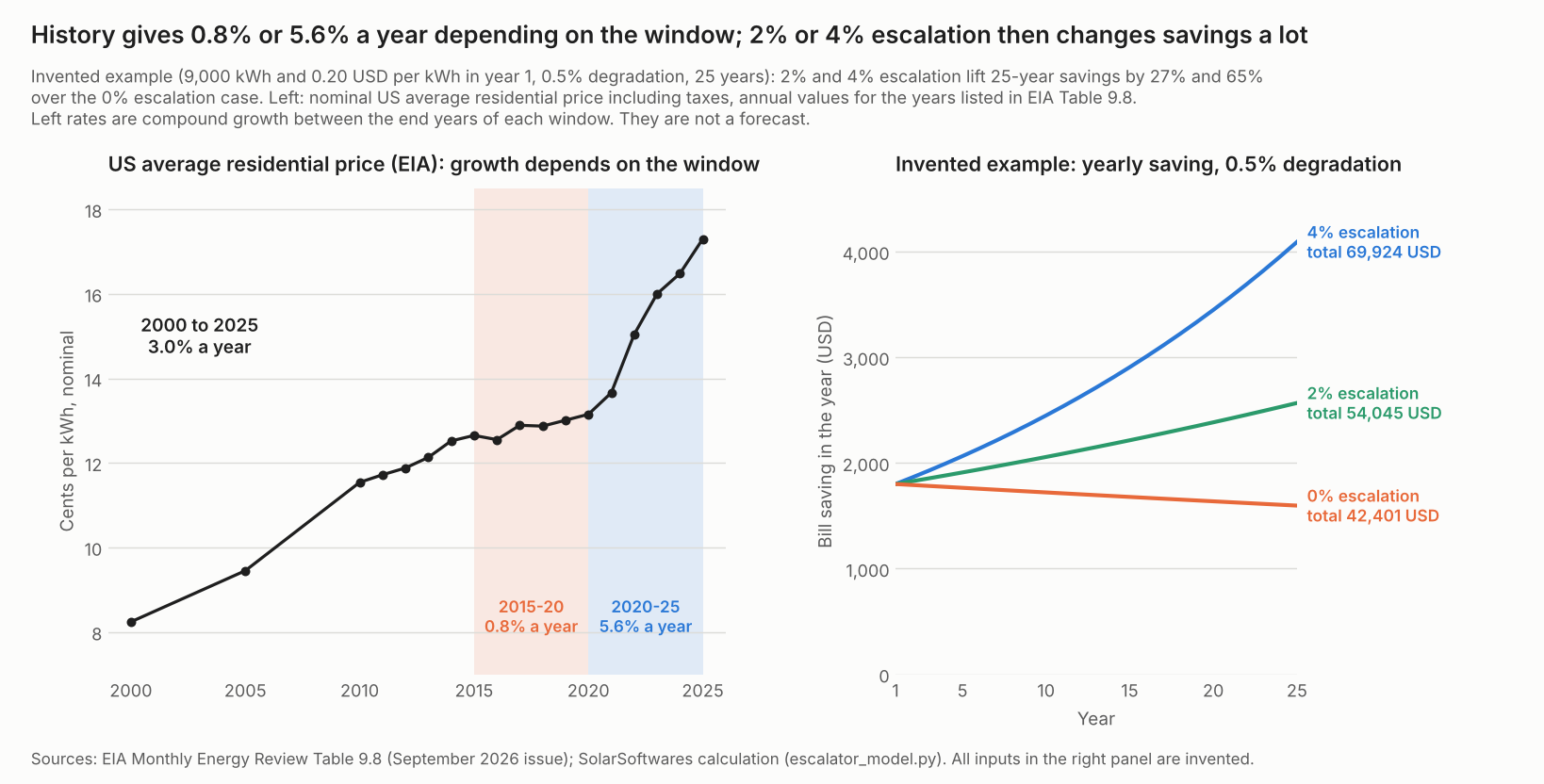
Figure 1. US residential prices grew 0.8% a year in 2015 to 2020 and 5.6% in 2020 to 2025 (EIA, nominal).
Year-1 saving is 9,000 × 0.20 = 1,800 USD. With no escalation and no degradation, 25 years give 45,000 USD. A hand sum confirms it. The year-25 price is 0.3217 USD per kWh at 2% and 0.5127 at 4%.
| Total saving over 25 years (USD) | Degradation 0% | Degradation 0.5% | Degradation 1% |
|---|---|---|---|
| Escalation 0% (reference) | 45,000 | 42,401 | 39,992 |
| Escalation 2% | 57,655 | 54,045 | 50,712 |
| Escalation 4% | 74,963 | 69,924 | 65,283 |
The next table adds year-25 saving, present value and the yearly change at 0.5% degradation.
| With 0.5% degradation | Year-25 saving (USD) | 25-year total (USD) | Present value at 5% (USD) | Yearly change in saving |
|---|---|---|---|---|
| Escalation 0% (reference) | 1,596 | 42,401 | 24,201 | minus 0.50% |
| Escalation 2% | 2,567 | 54,045 | 29,363 | 1.49% |
| Escalation 4% | 4,091 | 69,924 | 36,177 | 3.48% |
Moving the rise from 2% to 4% adds 15,878 USD at 0.5% degradation. Moving degradation from 0% to 0.5% at a 2% rise removes 3,609 USD. The ranges differ in size, so this is not a ranking of inputs.
Discounting shrinks the gap: the 4% case is worth 36,177 USD in present value, which is 52% of its total.
Utility rate escalation calculator
The presets reproduce the tables above. A second block turns two prices into a compound yearly rate, so you can check history. It warns about blank, zero, negative or out-of-range inputs instead of returning a result. It is a design aid, not financial advice.
How solar software handles utility rate escalation
Aurora, HelioScope, OpenSolar and SAM’s PySAM module each document an escalation input. Only OpenSolar prints a default value, and the Aurora and SAM pages do not say whether the rate is real or nominal.
| Software | Escalation input? | Where set | Source |
|---|---|---|---|
| Aurora Solar | Yes | Settings > Utility and tax rates, with a project override | Aurora help, financial analysis overview and utility rate escalation settings (no date shown, checked 28 October 2026) |
| HelioScope | Yes | Financial Templates, Modeling | HelioScope help, Financial Modeling Glossary (no date shown, checked 28 October 2026) |
| OpenSolar | Yes | Control > Design & Hardware > Setback & Design Settings > Simulation Settings | OpenSolar support, "How to adjust your simulation settings" (no date shown, checked 28 October 2026) |
| SAM (PySAM module) | Yes | Input rate_escalation in the NREL-PySAM Utilityrate5 module | NREL-PySAM 4.0.0 documentation, Utilityrate5 (checked 28 October 2026) |
- Aurora Solar: "Utility escalation rate". A second help page describes a default rate with minimum and maximum limits, and location rates for US states and Canadian provinces. No default value is printed on the pages read. Real or nominal not stated.
- HelioScope: "Utility Cost Escalator" with an Annual Escalation Rate field: it "Increases utility prices each year by the rate set in this field". PPA financing has its own escalation rate. No default printed.
- OpenSolar: "Utility Inflation / Price Inflation Annual (%)" is the annual increase in utility rates used in financial savings calculations. Printed default: 3% per annum. A separate Feed-in Tariff Inflation input covers feed-in tariffs.
- SAM (PySAM module): "Annual electricity rate escalation [%/year]". Set to 0 if not assigned. The page does not say real or nominal. The SAM desktop help is not covered here.
These inputs sit inside proposal and financial tools. To compare them, see the best solar proposal software, best commercial solar proposal software and best solar financial modeling software lists.
Common mistakes with utility rate escalation
FAQs
What escalation rate should a solar proposal use?
Start with a low, base and high case built from EIA’s US history, then swap in the customer’s own tariff history. That history spans 0.8% to 5.6% a year across two windows. Tool defaults differ: OpenSolar’s page prints 3%, Aurora lets an admin set a default with limits, and PySAM uses 0 if none is given.
Is the escalator in a PPA the same as utility rate escalation?
No. A PPA or lease escalator is a contract term. It sets what the host pays. Utility escalation is an assumption about the tariff. It sets what the host avoids. See the power purchase agreement page for the contract side.
Does escalation apply to exported power?
Not automatically. OpenSolar has a separate Feed-in Tariff Inflation input, so check whether your tool escalates exports at all, and whether your export tariff does.
Can the escalation rate be zero or negative?
Yes. EIA’s US annual average fell in 2 of the 15 yearly changes from 2010 to 2025. California’s 2025 average was below 2024. A 0% case is a fair test. The calculator accepts rates from minus 20% to 20%.
Related terms
- Degradation rate: the yearly fall in module output that offsets escalation.
- Solar lease: a fixed payment with its own contract escalator.
- Power purchase agreement: a price per kWh with a contract escalator.
- Payback period: the years of savings needed to repay the net cost.
Next step: set the escalation rate in a low, base and high case, then compare proposal tools that let you show all three.
Sources
All sources opened October 2026.
- Prices. EIA Monthly Energy Review, Table 9.8, October 2026 issue. EIA Electric Power Annual, Table 2.10. EIA Electricity Monthly Update, data for August 2026, released 23 October 2026.
- Software. Aurora, financial analysis overview and utility rate escalation settings. HelioScope Financial Modeling Glossary. OpenSolar, simulation settings. NREL-PySAM 4.0.0, Utilityrate5.
- Calculation. Worked-example inputs are editorial assumptions.
Last updated 30 October 2026. Next scheduled review: 30 January 2027.